Digging into species likelihood with eBird and DuckDB

In part 2 of this exploration we dug deep into how to answer the question "where do all the birders go?" We found many ways to make queries run very slowly on DuckDB but ended up hitting our initial goal of starting to use the EBD in production. Now, we're going to extend that further to see if we can show people how many birds might be likely in a given place and time.

Best practices when working with eBird data

I'll admit from the start that this is far more of a daunting exercise than the last one. The analysis part of the hotspot popularity was pretty straightforward: count the checklists and group them by the hotspot and month (though, that didn't stop me from making plenty of mistakes). The challenge there was more on the technical side of getting queries to run quickly and efficiently. This part will be much more challenging on both fronts. For one, answering the question of "which bird can be seen where" with any sort of correctness is quite hard. Second, doing this in a way that will work in production is not going to be easy.

One advantage that I do have this time around is the fact that the eBird team have spent a lot of time discussing and documenting how to go about this exact sort of analysis. I'll be borrowing heavily from their fantastic resource here on Best Practices for Using eBird Data.

A particular highlight I'd recommend going over is the various biases or imbalances that creep in when using citizen science data like eBird. I'll summarize briefly here, but it's very readable if you want to check it out directly. The underlying thing we're trying to measure is when and where a species of bird will be at any given point. We can't just know this, so we're forced to estimate this in some way. The data source we're using here is humans going out and writing down which birds they saw and how many. Many of them do this with a scientific mindset, but they're also humans with preferences and needs that influence when and where they do this. So we end up with lots of trends in the observations that are more human than avian. We humans prefer to bird on the weekends, during migration when there are plenty of birds, when the weather isn't horrendous and so on. And we tend to notice, well, more noticeable birds. A loud or beautiful bird song will get noticed better than an owl sleeping nearly invisibly at the top of a tree.

Writing a query for species likelihood

Bringing this to the task at hand, let's start with a naive analysis of species likelihood. We'll count the number of checklists in a hotspot for a certain month. Then we'll count how many times a species appeared on a checklist in that place. Dividing those we should get a rough idea of "what are the most likely birds to see then and there?"

Here's a quick way I got to this data, with the regular caveat that I've certainly made mistakes:

with
  total_checklists as (
    select
      extract (
        month
        from
          "OBSERVATION DATE"
      ) as month,
      "LOCALITY ID",
      count(distinct "SAMPLING EVENT IDENTIFIER") as total_checklists
    from
      ebird_ny."full"
    where
      "OBSERVATION DATE" > current_date - interval '5 year'
      and month = 8
      and "LOCALITY ID" = 'L165143'
    group by
      1,
      2
  ),
  species_checklists as (
    select
      extract (
        month
        from
          "OBSERVATION DATE"
      ) as month,
      "LOCALITY ID",
      "COMMON NAME",
      count(distinct "SAMPLING EVENT IDENTIFIER") as species_checklists
    from
      ebird_ny."full"
    where
      "OBSERVATION DATE" > current_date - interval '5 year'
      and month = 8
      and "LOCALITY ID" = 'L165143'
    group by
      1,
      2,
      3
  )
select
  "COMMON NAME",
  species_checklists,
  total_checklists,
  species_checklists / total_checklists
from
  total_checklists
  join species_checklists using ("LOCALITY ID", month)
order by
  species_checklists desc
limit
  10

There's probably a quicker way to write that too, but using something like window functions gets a little tricky since I don't want to just add up the checklists counts for all species. Instead I want the unique list of checklists. Anyways, here's what that returns:

COMMON NAME	species_checklists	total_checklists	likelihood
Laughing Gull	593	669	0.8863976083707026
Mute Swan	548	669	0.8191330343796711
Great Egret	539	669	0.8056801195814649
Osprey	533	669	0.796711509715994
Double-crested Cormorant	532	669	0.7952167414050823
Gray Catbird	527	669	0.7877428998505231
Canada Goose	519	669	0.7757847533632287
Mallard	516	669	0.7713004484304933
Northern Mockingbird	509	669	0.7608370702541106
Snowy Egret	506	669	0.7563527653213752

(if the numbers seem high that's cause the totals are across the past 5 years or so of data)

Sorted the other way (least popular first) we have these:

COMMON NAME	species_checklists	total_checklists	(species_checklists / total_checklists)
Whimbrel	1	669	0.0014947683109118087
Monk Parakeet	1	669	0.0014947683109118087
Calidris sp.	1	669	0.0014947683109118087
Wilson's Warbler	1	669	0.0014947683109118087
Piping Plover	1	669	0.0014947683109118087
Hooded Warbler	1	669	0.0014947683109118087
White-faced Ibis	1	669	0.0014947683109118087
Black-throated Green Warbler	1	669	0.0014947683109118087
Dickcissel	1	669	0.0014947683109118087
Tricolored Heron	1	669	0.0014947683109118087

This matches my gut level instincts of what might show up at Jamaica Bay in August. But there are some additional steps we should consider.

The main one is that we can't naively assume that most people were trying to do complete checklists. Put another way, if someone birded for 2 minutes in Jamaica Bay and saw 3 species, a Laughing Gull, a a House Sparrow and an Osprey, we should not assume that a Mallard wasn't in Jamaica Bay that day. The eBird docs go much further into what to think about here, but being able to do this conversion, in the right way, is one of the most valuable aspects of eBird and why complete checklists are so valuable to science!

Oh and also we probably shouldn't factor in Calidris sp. type reports either. So let's apply a few recommended filters:

• we'll only include species
• no incidental checklists
• keep it under 10km

Last, I'll throw in a distinct at the top for 2 reasons. 1, this should condense "shared" checklists down to only 1 report per species. 2, I think this will also collapse sub-species into the regular species name. Both of these are definitely areas to followup on, though I hope it'll be good enough for now.

I'll just define those in a new input_data expression to make it easier to keep things consistent:

select
    distinct -- distinct is here to exclude duplicate (shared) checklists
    extract (
    month
    from
        "OBSERVATION DATE"
    ) as month,
    "LOCALITY ID" as locality_id,
    "SAMPLING EVENT IDENTIFIER" as checklist_id,
    "COMMON NAME" as common_name
    from ebird_ny."full"
    where
    "OBSERVATION DATE" > current_date - interval '5 year'
    and CATEGORY = 'species'
    and "PROTOCOL TYPE" in ('Stationary', 'Traveling')
    and "EFFORT DISTANCE KM" < 10

Once we have that, we can now run this across all the hotspots for August (I'm using a narrow New York only dataset to make this easier). This way we can see something like "which hotspot has the highest number of species likely to be found at it?" And we get something surprising:

month	LOCALITY	locality_id	common_species	uncommon_species	total_checklists
8	St. Lawrence River Dike Trail at Richard's Landing	L1810696	100	0	12
8	Freshkills Park--North Park (Phase l)	L27548440	96	0	6
8	Ulster Park	L16301078	95	16	34
8	Jamaica Bay Wildlife Refuge	L165143	94	40	619
8	Montezuma NWR--Towpath Rd.	L266832	93	54	70
8	Montezuma NWR--Knox-Marsellus and Puddler Marshes	L679571	92	14	44
8	Lower La Chute River & Ticonderoga Marsh	L4910422	91	0	11
8	Spring Farm Nature Sanctuary	L6624443	89	0	16
8	River Rd. marshes and RR tracks	L2457005	89	0	15
8	Columbia University, Nevis Laboratories Environs	L27674356	89	0	16

The top hotspot is only one with 12 checklists in it. I haven't checked those checklists myself to see if they're valid, but there's nothing to say there's anything wrong with something like this. There are plenty of very rich hotspots out there that don't get visited that often. Still, it seems less than ideal if we'd rank this spot as more rich than something like Jamaica Bay where not only does it have a similar count of species, but we're also far more certain of the numbers you can see there. We're gonna need... statistics for this.

Error rate / confidence

What I think I really want here is not necessarily a way to alter the number of species we show for lower frequency hotspots. Instead, we really just want to return additional data alongside it that shows how confident we are in the data. It's been a long while since I was in stats class and unfortunately I'm drawing a bit of blank on how best to model data like this. What's confusing to me is that we're not really dealing with "random" data per se. A birder seeing 90 species at a location over 3 hours is a good sign that there's going to be a lot of species at that location. But it's not obvious to me how to rate that finding if 100 other birders hit that level, or if no one else does. It would feel like a mistake to throw that observation out, or even to water it down with 10 other quicker trips if they only spent a few minutes and recorded 10 species.

I think what I'll do for now is do a very rough "error" calculation (rough cause I'm truly not sure if it's right), and return that to my map alongside the unmodified count of "common" species. Here's how I calculate that:

sqrt(common_species) / total_checklists

Getting this to the front end

Now, I had planned originally on making another table for this data, but I think with the learnings from last time, it might make sense to just throw this data into our existing popular hotspots table. It will definitely increase the table size, but I won't have to, hopefully, worry too much about performance with a new JOIN.

But, let's just see how this looks now. I haven't talked much about the frontend side of displaying things in this series, and that's mostly cause I haven't thought too much about it. It's mostly been me (Claude) copy and pasting the existing map code I have here. I don't want to do this forever, but it's been "good enough" for now. So let's keep doing that.

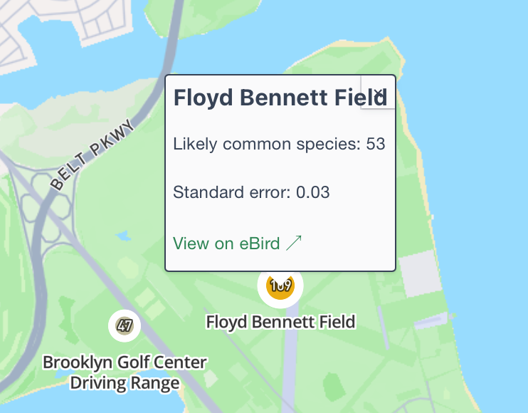
So with a decent prompt, we're up and running... except these numbers are a bit off. Why is Floyd Bennet showing 109 on the map but 53 in the tooltip?

Looking at the DB for that location and month:

┌─────────────┬─────────────────────┬───────────────────────────────────┬────────────────┐
│ locality_id │    locality_name    │ avg_weekly_number_of_observations │ common_species │
│   varchar   │       varchar       │              double               │     int64      │
├─────────────┼─────────────────────┼───────────────────────────────────┼────────────────┤
│ L152773     │ Floyd Bennett Field │                 7.869565217391305 │             53 │
│ L152773     │ Floyd Bennett Field │                 7.869565217391305 │             93 │
│ L152773     │ Floyd Bennett Field │                 7.869565217391305 │             70 │
│ L152773     │ Floyd Bennett Field │                 7.869565217391305 │             55 │
│ L152773     │ Floyd Bennett Field │                 7.869565217391305 │             63 │
│ L152773     │ Floyd Bennett Field │                 7.869565217391305 │             92 │
│ L152773     │ Floyd Bennett Field │                 7.869565217391305 │             71 │
│ L152773     │ Floyd Bennett Field │                 7.869565217391305 │             85 │
│ L152773     │ Floyd Bennett Field │                 7.869565217391305 │             62 │
│ L152773     │ Floyd Bennett Field │                 7.869565217391305 │            109 │
│ L152773     │ Floyd Bennett Field │                 7.869565217391305 │             67 │
│ L152773     │ Floyd Bennett Field │                 7.869565217391305 │             59 │
├─────────────┴─────────────────────┴───────────────────────────────────┴────────────────┤
│ 12 rows                                                                      4 columns │
└────────────────────────────────────────────────────────────────────────────────────────┘

We should not have 12 rows for this. Oh the ole 1:many accidental JOIN issue. I'm creating my final table like so:

SELECT
  locality_id,
  month,
...
FROM
  localities l
  JOIN hotspot_popularity hp USING (locality_id_int)
  LEFT JOIN hotspots_richness hr using (locality_id_int)
...

The join on the ID is fine, but I forgot I need to make sure the same month is used for popularity and richness. This ought to fix it:

LEFT JOIN hotspots_richness hr using (locality_id_int, month)

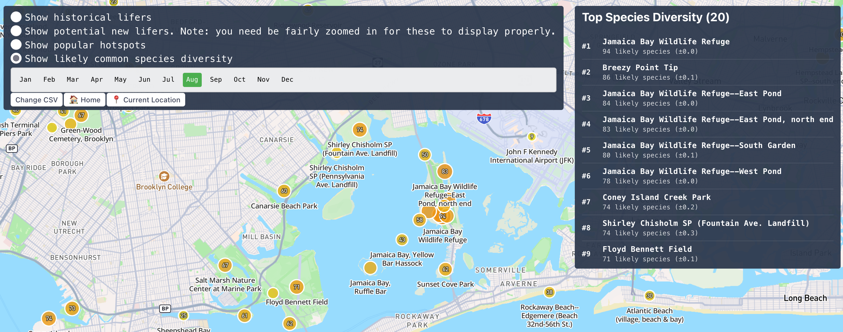
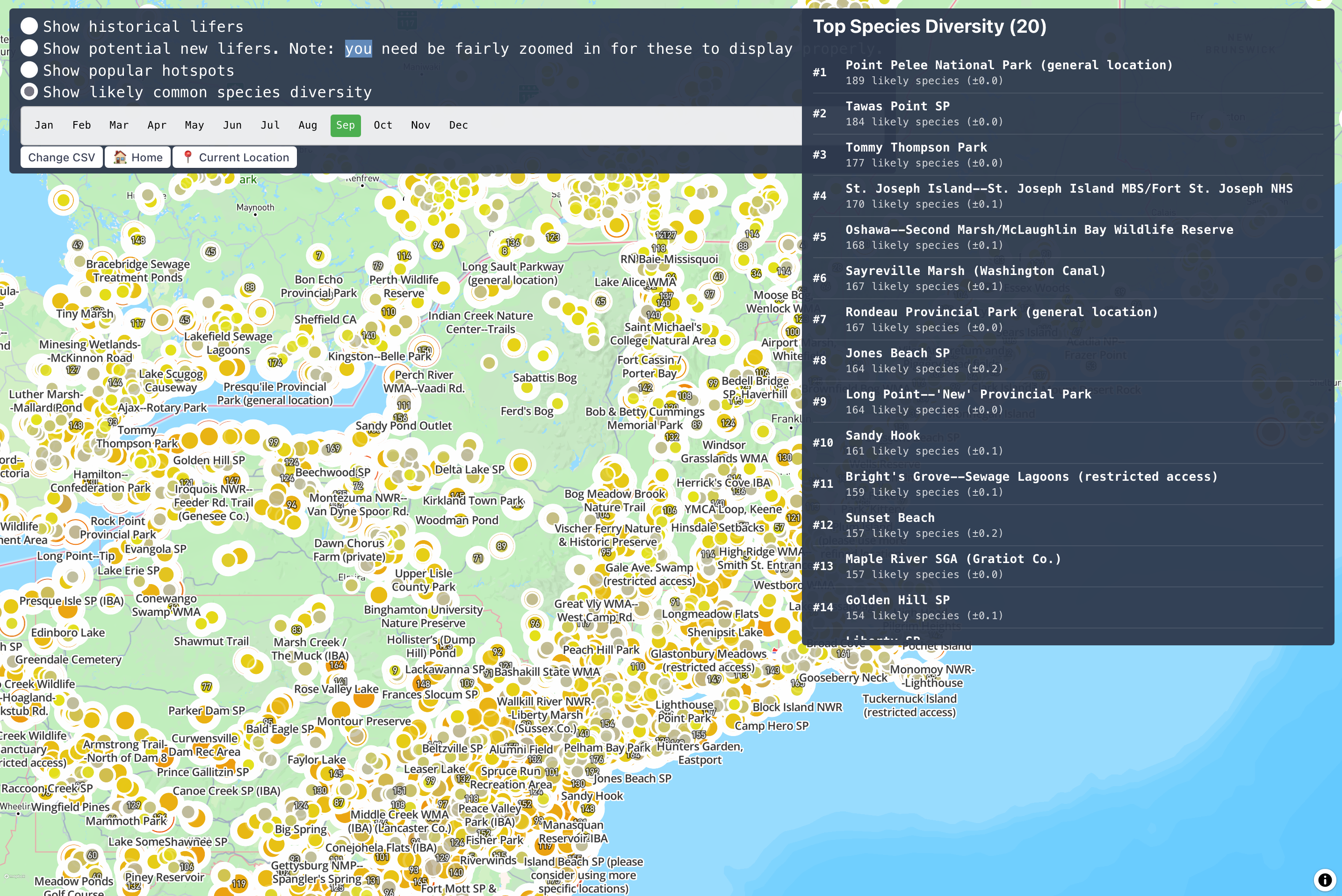
Zooming out a bit things are looking overall pretty good. It's hard to say how accurate this is... I'm learning from just looking around on the map which hotspots really shine at which time of year. I'm also struggling a bit to figure out how best to show an error bar or confidence interval at this level. Should I fade out lower confidence hotspots? Should I make the edges blurrier? Should I de-saturate them?

For now I think I'm going to focus on the more core problem of making sure this data is accurate. If I quickly compare some hotspots it seems my methodology is vastly under-counting compared to eBird. It's been fairly hard for me to figure out how eBird and Merlin calculate the numbers here. I've seen that for a species to not be a yellow dot, it has to appear on 6% or more of checklists. And that's actually what I used initially in my data. However, if I actually look into the eBird mobile species under "Likely" for a hotspot they include these yellow dots. So maybe I should include them in mine? Or really what I want to do is to include both?

Adding those numbers in brings my numbers much closer to eBird's. I think it also makes since to display both in the tooltip. Maybe I can even add an option shortly to toggle the map from displaying either just common birds or both common and uncommon?

Scaling this up

Before going too much further though I want to stop and check in on the performance of this. I'm a little wary of adding too much more data if I can't actually deploy it. I do most of my development off of a more limited NY-only dataset. This is plenty for testing and poking around, but I still need to run the full thing to make sure I'm not gonna drain the bank on storage fees.

The first run of this... wasn't promising. I very quickly drained my computer memory and the spillover disk storage. I hadn't taken a cleanup or refactoring pass through the likelihood query, so I did quick look through to remove some extraneous columns and CTE's. One quick snack break later... and no luck. Still running out of space. Off to the DuckDB docs again!

The docs were helpful as always, but there weren't too many tricks I hadn't already tried. The job is already getting as much memory and disk space as I can provide and I'm not going anything woefully incorrect with my setup from what I can tell. A few things that did stick out to me: when I initially set up the full dataset, I didn't do anything to help optimize by using the correct types, sorting by timestamps or filtering out data or columns I'm not going to use. That's probably long overdue here so I set about trying to define a more intermediate table to work off of. Unfortunately, with me stuck with the already too-large dataset on my hard drive I wasn't left with enough room to spin off a new one, pruned though it might be. Thankfully, I already needed to regenerate the underlying dataset with the latest data from July so we might as well take that on and clean up and format the data a bit more as we go.

A long side quest on better data import

Back in Part 1, I was just trying to get to the point of being able to query the EBD in a DuckDB dataset. It was a slow but fun journey, but I'd only done this once. Thus, my methods of doing so were sloppy at best and I knew the next time I was going to do this I should take a few passes and cleaning up what I was going and also making it a bit more efficient. This latter part really piqued my interest this time around, almost certainly to a negative degree. I had the external disk space to just do this in a slow, but sure way, converting the compressed form into an uncompressed TSV and then into a DuckDB database. Still, that felt quite wasteful and slow (in reality it would just mean firing off two scripts before going to bed one night and then waking up to a fresh dataset ready for use). So, like many times before, I set off to spend a bunch of mostly unnecessary time speeding this up and making it more efficient.

The core of what I didn't like about the old flow was the necessity of reading through the data 2 or even 3 times to get to a working DuckDB:

1. Once to un-tar the files (I'm not entirely positive if this requires reading all of the underlying bytes)
2. To decompress the compressed TSV file inside of that TAR
3. To load that TSV file into DuckDB

What would be great is if we could go from the .tar file to the full DB in one step. Theoretically I knew this was possible but I wasn't sure how feasible it would be with the existing tools I had. Something that gave me early confidence was the fact that DuckDB can read directly from stdin when invoked from the command line like so:

cat ebird.tsv | duckdb -c "SELECT * FROM read_csv('/dev/stdin')"

Neat! All that's really needed then is to selectively read and decompress the .gz file inside the .tar and pass that into DuckDB. Overall this was pretty straightforward and it wasn't long before I had a simple working solution. One aside here is that I did all of this myself in bash as a first pass, but then opted to let Claude Code then take a pass at polishing the script to have more logging, a progress bar using pv and good timing tracking. Claude Code really seems at its best in moments like this where I have a very clear overall direction for what I want to do, but can rely on it to introduce extra details like args, or logging that would be finicky or frustrating for me to get just right with my intermediate bash knowledge. Here's how it looked once I had it up and running for real:

 % ./queries/parse_ebd.sh ebd_relJul-2025 ./dbs/ ./dbs/
Starting eBird data processing at Sat Aug 30 09:28:23 EDT 2025
Processing: ebd_relJul-2025
Output database: ./dbs/ebd_relJul-2025.db
[09:28:23] Removing existing database file...
[09:28:23] Database file removed
[09:28:23] Starting data extraction and processing...
  - Extracting ebd_relJul-2025.txt.gz from tar archive
  - Archive size: 198.9G
  - Compressed .gz file size: 198.9G
23.1GiB 0:11:20 [34.5MiB/s] [==>                 ]  11% ETA 1:25:42

I'm pretty happy with how this script came together! It's much more efficient with disk space and quicker than doing this in 3 steps. It takes about 60-90 minutes to complete which is the difference between leaving it for a night vs leaving it for a run or a long walk. Here's the full version if you care to look.

It wasn't all success, though. One important goal I had for this refactor was to introduce better ordering at this stage. DuckDB really emphasizes in their docs and blogs the importance of table ordering for good performance, especially in this great article: https://duckdb.org/2025/05/14/sorting-for-fast-selective-queries.html. Naively, I thought I could just throw in an order by observation_date at the end of my new script and get this for free. However, this just resulted in all of the free disk space on my machine getting eaten up at an alarmingly fast pace. I think what was going on here is that DuckDB had to basically read in the entire contents of the DB into either memory or spillover disk space to determine the right order before it could begin to start committing anything into the more space-efficient DB.

Fresh data but no progress

So, while it was good to have a much better import script and the latest EBD data, I still didn't feel like I was getting any closer to being able to generate the full data I wanted here if I couldn't actually set up ordering. Now the challenge is entirely about how to get this data ordered in a reasonable way. I searched around for ideas about how to order this in place, but didn't find anything mentioning this as a feature of DuckDB. I couldn't just write a new query to just "create a new table with everything in the old table but order it" since I'd just run out of disk space again.

Thankfully, while on a walk a rather simple solution occurred to me. Just do this in batches. I can easily read a "chunk" of the old dataset, push it into a new DB and order it there. Since I'm only working with a portion of the data at a time then I shouldn't eat up all the available disk space, just what's necessary to sort the portion of data I chose. And, if disk space gets precious, I can actually just delete those rows from the old DB once I insert them so I'm not actually net adding more data to my machine.

I thought for a few minutes on the right elegant solution to reliably and repeatedly split my data up before opting to just do it by the month of the observation. In hindsight I think this might've been really silly though... I want to be sorting by observation date but if I'm doing this across months then I think I'm probably having to read across wildly different chunks or pages of the data? In any case, the logic of this was pretty straightforward.

First, create the new DB copying the schema over from the old DB:

CREATE TABLE ebd_sorted AS
FROM
  ebd_unsorted.ebd_full
WITH
  NO DATA;

Then, just iterate through the months of the years and push them into the new DB:

months_of_year=(1 2 3 4 5 6 7 8 9 10 11 12)
for MONTH in "${months_of_year[@]}"; do
  duckdb path_to_output_db <<EOF
    INSERT INTO
      ebd_sorted
    FROM
      ebd_unsorted.ebd_full
    where
      extract month = $MONTH
    ORDER BY
      observation_date;
EOF
done

Thankfully when used like this DuckDB will just compute the percentage for you:

[07:58:42] Processing month: 1
100% ▕████████████████████████████████████████████████████████████▏
[08:05:58] Processing month: 1 completed
Total execution time: 7m 16s
[08:05:58] Processing month: 2
10% ▕██████

Un-thankfully, it's entirely inaccurate when you're adding sorting at the end. The first time I ran this I crashed my machine since I had very little storage left. Deleting a couple dozen old or broken DuckDB's fixed this and the second time this ran to completion in about 90 mins. That's honestly a bit surprisingly slow, though a bit reason for that could be my quite silly chunking strategy. Another confusing thing is that the insertions get faster rather than slower in later batches. You can see there the first insertion took 7+ minutes while the last month took less than 5. I'm not entirely sure why this might be. I would have assumed DuckDB would have to do more work at the end to figure out the right insertion order?

In any case this worked, but leaves a lot to be improved upon in future iterations:

• picking a better chunking strategy
• figuring out how the raw TSV is sorted if at all. If it is it'd be great to use that for my chunking strategy
• the dream: could I figure out a way to merge this step in with the prior one so that I'm iteratively sorting the data as I read it in from the TSV?

Here's the script if you care to take a look!

Back to the real purpose

The prior few sections were over a few days of intermittent work, so I was a little fearful that all of that might have been a pointless adventure into premature optimization that went actually nowhere in terms of fixing the actual problem: being able to show species likelihood across the full data set.

Thankfully, the sorting did appear to pay off and the first run with the full data set was successful! This species richness table creation is still painfully slow, but it finishes:

  Creating localities table with spatial columns... ✅ Created in 13.1s!
  Creating taxonomy table... ✅ Created in 0.1s!
  Creating hotspot popularity table... ✅ Created in 61.0s!
  Creating hotspots richness table... ✅ Created in 525.9s!
  Creating localities_hotspots optimization table... ✅ Created in 7.2s!
  Dropping hotspots richness table... ✅ Dropped in 0.2s!

Nearly 10 minutes to create that one table, but that's a small price to pay to be able to see this many hotspots on a map at once!

Conclusion

I really need to take a pass now at cleaning things up on the display side of this. I also should absolutely be limiting this query... each one of these runs returns 20MB of data. But, I think this is a nice place to wrap up this post. I'm not entirely certain where I'll go from here next. There are more than a few places to explore:

• I'd love to be able to show more information to users about not just the number of species but characteristics about them.
• I'd love to be able to use this data to now compute "where can I see the most lifers"? I'm already showing that on another page, but it's using the eBird API and is woefully slow to run. This is going to be hard though because I can't just aggregate the species count for efficiency's sake. I'll need to report back the actual list of species for the hotspot, which would add a whole lot of data.
• My hope here isn't to have a bunch of different maps with disparate information on them. Instead, I'd like to support a single view for "Where should I go?" that takes into account richness, popularity, lifers to various data points on a hotspot.
• Most of all, I really need to take a pass on polishing things end to end so I can actually share this with some birding friends and have them use it!